Artificial Neural Networks: The Basics

Artificial Neural Networks (ANNs) exist in a fascinating intersection of neuroscience and machine learning, giving rise to powerful systems that can emulate intelligent behaviors. This note covers the essential glossary and theory behind this powerful technology.

A Network of Neurons

flowchart LR
sigma((Σ + bias))
x1((Input1)) -- Weight1 --> sigma
x2((Input2)) -- Weight2 --> sigma
xn((Inputn)) -- Weightn --> sigma
sigma --> activation((Activation\nFunction))-->output((Output))

The basic building block of an ANN is the neuron. Just like in biology, an artificial neuron consists of multiple input nodes and a single output node. Neurons are connected in multi-layer networks, where an output from one neuron becomes an input to the next. The layers that lie in between the input layer and the output layer are referred to as the hidden layers, and a network that has more than a single hidden layer is referred to as a deep network. The network can be arranged in many different architectures, depending on the intended application. In this note, we will focus on a basic feed-forward architecture, commonly referred to as a multilayer perceptron (MLP). We will expand the concepts to other architectures in a future note.

The connections between each of the input nodes and the output node in a neuron carry weights. When a neuron network operates in a forward direction, i.e., to generate a prediction, the values of the input nodes are multiplied by their weights, summed, and then a bias term is added. This raw output of a neuron (often denoted by z) is then passed through an activation function, which is usually a non-linear function that remaps z on to a more convenient or meaningful scale (usually 0 to 1). The resulting final value of a neuron is called it’s activation (in many sources the usage of this term also includes the 0th layer inputs). It can be shown that the combination of linear weighted sum equations and the non-linear activation functions allows ANNs to act as universal function approximations. ANNs are most commonly designed to solve classification problems, but there are designs that allow regression-like value prediction as well.

Mathematically, a layer of neurons can be represented as: $$ \vec{a}^{l+1} = \sigma(z^{l}) = \sigma(\matrix{W} \vec{a}^{l}+\vec{b}^l) \tag{1.1} \label{neuron} $$

where l is the layer number, a are the activations of a given layer, W is the weights matrix, b are the scalar bias terms, and \( \sigma\) is an activation function. See here for a quick refresher on linear algebra.

On occasion, we will need to zoom in on to a specific neuron, so here is the same equation that is stated in terms of the activation of the j’th neuron in layer l: $$ a^{l+1}_j = \sigma (\sum w_{jk}^l a_k^{l} + b_j^l) \tag{1.2} \label{neuron2} $$ where k is the index of a given input. As an additional note, in our notation the capital L will be used to represent the total number of layers, and when used as an index, will refer to the output layer.

The weights and biases are the parameters of an ANN model that get adjusted through training. Training brings the weights to represent an input state that most corresponds to a specific output. Prior to training, the parameters are randomly initialized, and are then algorithmically adjusted to improve the model’s fit of the data.

For simplicity, the bias parameters can be treated as weights with a constant activation term of 1. Thus, it is common that both types of parameters are implicitly referred to as weights.

In most ANN architectures, the same set of inputs is fed to the many neurons contained in the next layer. That means that each of the neurons in a given layer can have a different weight assigned to the same input from the previous layer. In a sense, the weight reflects how “important” an input is to a specific neuron. By prioritizing specific sets of inputs, a neuron essentially picks out and focuses on a specific feature of the inputs. Successive layers are able to recognize more complex features, since they aggregate and recombine features from past layers, a phenomenon referred to as the feature hierarchy. Through this buildup of feature complexity, ANNs are able to perform automatic feature extraction and discover complex latent structures in data.

Activation functions

An activation function is a non-linear function that remaps z on to a more meaningful or operable scale, often between 0 and 1. The sigmoid is a popular activation function used in the hidden layers of simpler networks:

$$ \sigma(z)=\frac{e^z}{1+e^z} \tag{2} \label{sigmoid} $$

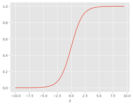
The sigmoid is a poster child of non-linear functions, but it presents an issue when training larger ANNs. When a specific weighted sum input (z) results in an activation output that is embedded far in one of the two plateau ranges of the function (i.e., when input/output of the function is far from the sigmoid inflection point), “getting out” of this plateau using an step-wise numerical optimization algorithm can be very slow. This is often referred to as neuron saturation, a detrimental behavior where changes in the input data do not lead to corresponding changes in the output, reducing the network’s sensitivity to variations in the data.

Other activation functions that are frequently used for hidden layers include tanh and ReLU, with the later one being a very popular choice for deep networks.

The output layer often uses different activation functions. Softmax is a function that is often applied for multi-class classification. It is essentially a sigmoid function that acts on a vector of z values and returns a vector of “probabilities”, where all values add up to 1.

$$ softmax(z)_i = \frac{e^{z_i}}{\sum_{j=1}^Ne^{z_j}} \tag{3} \label{softmax} $$

where N is the number of outputs.

Argmax is another specialized function, which aims to “collapse” the probability distribution created by something like softmax. It acts by setting the maximum value of the z vector to 1, and everything else to 0.

$$ argmax\left(\begin{bmatrix} 0.1 \\ 0.7 \\ 0.2 \end{bmatrix}\right) = \begin{bmatrix} 0 \\ 1 \\ 0 \end{bmatrix} \tag{4} \label{argmax} $$

Training

Cost functions

The progression of learning is measured by the minimization of a cost function (also often referred to as the loss function). The cost function is a layer of complexity above the network. A cost function consists of:

• Inputs: weights and biases of the network
• Parameters: a set of training examples and the corresponding predictions of the ANN.
• Output: the cost

A basic cost function is the mean squared error (MSE):

$$ C=\frac{1}{n}\sum_{i=1}^{n}(y_{train}-y_{pred})^2 \tag{5} \label{mse} $$ where \( y_{train} \) and \( y_{pred} \) are corresponding pairs of training and ANN-predicted outputs, and n in the number of such pairs. While MSE is good for illustrative/educational purposes, it has significant performance issues, and is rarely used in practice.

In modern ANN architectures, especially those used for multi-class classification problems, a more common cost function is the cross-entropy loss. The function comes from the field of information theory, and (roughly speaking) allows us to calculate differences between two probability distributions. In ANN, the cross-entropy loss function takes the output vector of probabilities and calculates the distance to the vector of labels from the training set, which is also a probability set, except where all of the probability is usually concentrated in a single node.

Understanding the math behind Cross-entropy requires a solid background on the information theory, which is out of the scope of this note. The exact form of the cost function depends on the structure of the network (specifically, the output layer). A general form of the equation that is used in the context of ANNs can be represented as:

$$ C = - \frac{1}{n} \sum_x \sum_j(y_j \ln a^L_j + (1-y_j) \ln (1-a^L_j)) \tag{6} \label{cross_entropy} $$ where n is the number of training examples, consisting of the inputs (x) and corresponding true values or labels (y), and a is the model-derived activation of the output neuron.

The cross-entropy cost function has a useful property: when calculating it’s gradient (the importance of which will be described in the next section), it does not depend on the derivative of the activation function. Thus, it can cancel out any slowdowns in learning caused by “plateau traps” within activation functions (like a sigmoid).

Regularization

The flexibility of ANN models is both a boon and a detriment. The large number of parameters available to ANN models make them very prone to over-fitting. Regularization is a set of techniques used to limit the degrees of freedom available to the model to safeguard against the tendency to shift from genuine learning to mere memorization of noise.

Norm-based regularization techniques, like L1 and L2 regularization, approach the task by trying to reduce the effect of weight decay: an unbounded growth of weight values due to the selection pressures excreted during training. By introducing a new pressure to keep the weight values low we can limit the excessive flexibility of the model. This is achieved by adding a weight based cost term into the overall cost function.

L1 regularization: $$ C = X + \frac{\lambda}{n}\sum_w |w| \tag{7.1} \label{l1_regularization} $$

L2 regularization: $$ C = X + \frac{\lambda}{2n}\sum_w w^2 \tag{7.2} \label{l2_regularization} $$

where \( \lambda \) is a regularization hyper-parameter, and X is the non-regularized version of the cost function, e.g., cross-entropy loss from equation \( \eqref{cross_entropy} \). When the gradient of the regularized cost functions is calculated, L1 regularization causes the weights to decrease by a constant amount, whereas L2 regularization causes weights to decrease by a factor proportional to the weight value. As a result, L1 regularization ends up with prioritizing a small number of high-impact weights, whereas the L2 regularization results in a more even spread of weight values.

Dropout regularization involves randomly deactivating a specified subset of neurons (typically 20% to 50%) in each training mini-batch. By introducing noise and variability into the network training, dropout prevents neurons from relying too heavily on specific features in the training data, encouraging them to learn more robust and generalizable representations. Dropout can be viewed as a form of ensemble learning, where different sub-networks (formed by dropping different sets of neurons) are trained simultaneously, leading to improved generalization performance on unseen data. Dropout is especially useful in training large, deep networks, where the problem of over-fitting is often acute.

Another strategy to reduce over-fitting is to expand the training dataset by incorporating artificial noise or variability (e.g., rotating/skewing images by a small amount in vision tasks).

Gradient Descent

ANNs are routinely built with billions of parameters, and minimizing the large cost functions needed for their training is no easy task. Finding an analytical minimization solution using standard calculus is not feasible in any practical application (it’s one of those cases when the analytical solution is more computationally costly than a numerical approach). But it can be achieved using the method of gradient descent, an iterative optimization algorithm used to minimize a function by taking steps in the direction of steepest downward change along the function profile.

The gradient is a differentiation operation that takes in a scalar-valued multi-variable function and returns a vector-valued function, i.e. a function that returns a vector at every point. A vector returned at any given point of the original function’s multidimensional response hyper-surface will point in the direction of its fastest increase, with the magnitude of the vector proportional to the rate of increase. In other words, the gradient provides information about how the cost function changes as you move through the parameter space. Mathematically, the gradient is a vector containing the partial derivatives of a multivariable function with respect to each of its variables. For a given ANN layer, the gradient is described by: $$ \nabla C = \begin{bmatrix} \frac{\partial C}{\partial w_1} \\ \frac{\partial C}{\partial w_2} \\ \vdots \\ \frac{\partial C}{\partial w_n} \end{bmatrix} \tag{8} \label{gradient} $$

As such, the gradient relates changes in the ANN parameters (w) to the corresponding changes in the cost function: $$ \Delta C \approx \nabla C \cdot \Delta w \tag{9} \label{gradient_change} $$

Being an iterative method, gradient descent takes small steps toward the minimization of the cost function. The size of this step is defined by a hyper-parameter called the learning rate (\( \eta \)), which controls the convergence speed and stability of the optimization process: $$ \Delta w = -\eta \nabla C \tag{10} \label{learning_rate} $$ The negative sign in the above equation allows us to move against the gradient, descending toward one of the minima of a function. The learning rate then defines the size of the step in each iteration \( \epsilon \):

$$ \epsilon = \Vert \Delta w \Vert = \eta \Vert \nabla C \Vert \tag{11} \label{step_size} $$

Gradient descent optimization usually starts off by setting the parameters of a minimized function (the cost function in our case) to random values. At each iteration, the gradient of the minimized function with respect to the parameters is computed, and the parameters are then updated in the opposite direction of the gradient using the following update rule:

$$ w^{\prime} = w - \eta \nabla C \tag{12} \label{update_rule} $$

where \( w^{\prime} \) are the updated parameter values. The update iterations are applied until a stopping criterion is met, such as reaching a maximum number of iterations or observing negligible improvements in the objective function.

In standard gradient descent, the gradient is calculated for every training example at every step towards the minimum, and the updates to the model parameters are made based on the average gradient. This becomes too costly given the number of parameters and training examples involved in training of ANNs. More commonly, the Stochastic Gradient Descent (SGD) variant of the algorithm is used, where the gradient is estimated using a small sample (a mini-batch) of randomly chosen training examples. On each iteration, a new mini-batch is selected, the estimate of the gradient is calculated and the model parameters are updated much more frequently. This goes on until all of the training data is exhausted. This denotes a training epoch, and training usually continues for multiple epochs, until the stopping criteria are encountered. While using a small subset of training data does not reveal us a true gradient at every iteration, turns out it gives us a pretty decent approximation. As a result, SGD converges to a solution much faster than regular Gradient Descent, and also happens to be less prone to over-fitting due to the inherent noisiness of random sampling.

Backpropagation

We’ve explained how Gradient Descent uses the gradient to iteratively minimize the cost function, but we have (conveniently) said nothing about how to calculate the gradient in the first place! This is where the backpropagation algorithm comes in. It allows us to calculate the gradient of the cost function relative to the weights and biases of the ANN model in an iterative fashion, moving backwards from the output to the input layers.

Deriving Backpropagation equations

Let’s explore the equations behind the algorithm. The equations may seem complex, but in reality it all boils down to the application of the derivative chain rule.

Quick Refresher of the Chain Rule: $$ f(g(x))^\prime = f^\prime (g(x)) g^\prime (x) \tag{13.1} \label{chain_rule_prime} $$ or in Liebniz’s notation: $$ \frac{dz}{dx} = \frac{dz}{dy} \cdot \frac{dy}{dx} \tag{13.2} \label{chain_rule_leibniz} $$

We will begin by introducing a term \( \sigma \) that represents the partial derivative of the cost function with respect to the weighted sum (z) of the j’th neuron in the l’th layer. This quantity is commonly referred to as an “error”, and it is a convenient starting point to start our derivation of the gradient equations.

$$ \delta_j^l = \frac{\partial C}{\partial z_j^l} \tag{14} \label{error_z} $$

Using the chain rule, we can express the error term relative to the weights in a given layer:

$$ \delta^l_j = \frac{\partial C}{\partial w^l_{kj}} \frac{\partial w^l_{kj}}{\partial z^l_j} \tag{15.1} \label{bp_grad_weights_init} $$

We can rearrange equation \( \eqref{neuron2} \) to express it in terms of the individual weights:

$$ w^l_{kj} = \frac{1}{a^{l-1}_k}(z^l_j - b^l_j) \tag{15.2} \label{bp_grad_weights_w_term} $$

This, in turn, allows us to calculate the partial derivative of the weights relative to the weighted sum of the neuron:

$$ \frac{\partial w^l_{kj}}{\partial z^l_j} = \frac{\partial (\frac{1}{a^{l-1}_k}(z^l_j - b^l_j))}{\partial z^l_j} = \frac{1}{a^{l-1}_k} \tag{15.3} \label{bp_grad_weights_w_term_dx} $$

By substituting the above into \( \eqref{bp_grad_weights_init} \), we can rearrange it to calculate the gradient of the cost relative to the weights:

$$ \frac{\partial C}{\partial w^l_{kj}} = a^{l-1}_k \delta^l_j \tag{15.4} \label{bp_grad_weights_final} $$

Deriving the gradient of the cost function relative to the biases follows a similar logic. Again, we express the error term relative to the biases in a given layer using the chain rule:

$$ \delta^l_j = \frac{\partial C}{\partial b^l_j} \frac{\partial b^l_j}{\partial z^l_j} \tag{16.1} \label{bp_grad_biases_init} $$

We rearrange equation \( \eqref{neuron2} \) in terms of the biases, and use it to calculate the partial derivative relative to the to the weighted sum of the neuron:

$$ \frac{\partial b^l_j}{\partial z^l_j} = \frac{\partial (z^l_j - \sum_k w^l_{kj} \sigma (z^{l-1}_k))}{\partial z^l_j} = 1 \tag{16.2} \label{bp_grad_biases_dx} $$

Substituting this and rearranging equation \( \eqref{bp_grad_biases_init} \) gets us:

$$ \frac{\partial C}{\partial b^l_j} = \delta^l_j \tag{16.3} \label{bp_grad_biases_final} $$

Great! We can now calculate the gradient relative to the weights and biases! Except, we need to know how to calculate the \( \delta \) term in each layer. Luckily, we can just rinse and repeat the same chain rule approach used above.

We can start with the output layer L, where the error term essentially represents the individual contribution of each of the output neurons to the cost. We will use the chain rule to represent the error in terms of the activations of the output layer:

$$ \delta^L_j = \frac{\partial C}{\partial \sigma (z^L_j)} \frac{\partial \sigma (z_j^L)}{\partial z_j^L} = \frac{\partial C}{\partial \sigma (z^L_j)} \sigma^\prime(z_j^L) \tag{17} \label{bp_error_output} $$

Lastly, let’s generalize the equation above to other layers. We will use the chain rule to calculate the error in any given layer relative to the error in the next layer:

$$ \delta^l_j = \sum_k \frac{\partial C}{\partial z^{l+1}_k} \frac{\partial z^{l+1}_k}{\partial z^l_j} = \sum_k \delta^{l+1}_{k} \frac{\partial z^{l+1}_k}{\partial z^l_j} \tag{18.1} \label{bp_error_next_layer_init} $$

As before, let’s calculate the partial derivative of the weighted sum in the next layer relative to the weighted sum in the current layer:

$$ \frac{\partial z^{l+1}_k}{\partial z^l_j} = \frac{\partial (\sum_j w_{kj}^{l+1} \sigma(z^l_j) + b^{l+1}_k)}{\partial z^l_j} = w_{kj}^{l+1} \sigma^{\prime}(z^l_j) \tag{18.2} \label{bp_error_next_layer_dx} $$

And substituting the above back into \( \eqref{bp_error_next_layer_init} \), we get:

$$ \delta^l_j = \sum_k \delta^{l+1}_{k} w_{kj}^{l+1} \sigma^{\prime}(z^l_j) \tag{18.3} \label{bp_error_next_layer_final} $$

Backpropagation steps

Now that we know how to calculate the individual components of the gradient, let’s put the whole algorithm into perspective:

1. A forward pass is performed to generate the outputs
2. The cost associated with the outputs is calculated
3. The error term in the output layer is calculated using equation \( \eqref{bp_error_output} \)
4. Moving backwards, the error term in all other layers is calculated using equation \( \eqref{bp_error_next_layer_final} \)
5. For each layer, the gradient of the cost function relative to the weights and biases is calculated using equations \( \eqref{bp_grad_weights_final} \) and \( \eqref{bp_grad_biases_final} \)
6. With the gradient calculated, the Gradient Descent equation \( \eqref{update_rule} \) is used to update each of the parameters

Exploding and Vanishing Gradients

In deep networks, the repetitive application of the chain rule often leads to a scenario where the gradient in each preceding neuron becomes either too small or too large. Mathematically, if the derivatives of the activation functions or weight matrices are consistently less than or greater than 1, the product of these derivatives can result in an exponential build-up, either resulting in an explosion or vanishing of the gradient. Both problems hinder effective training of deep neural networks but in opposite manners: one by making the gradients too small to effect meaningful weight updates and the other by making the gradients too large, causing unstable updates.

To avoid vanishing and exploding gradients in deep neural networks, several strategies are commonly employed, involving careful architectural choices, initialization techniques, and optimization methods:

• Proper initialization of weights is crucial in avoiding gradient problems. A common way to initialize weight values is to use Gaussian random variables with a mean of 0 and a standard deviation of \( \frac{1}{\sqrt{n}}\), where n is the number of input nodes of the network. This ensures that individual weight do not start at exceedingly high or low values.

• Using activation functions like ReLU (Rectified Linear Unit) and its variants, such as Leaky ReLU and Parametric ReLU, can significantly mitigate the vanishing gradient problem. ReLU does not saturate for positive values, which helps in maintaining gradients. However, ReLU can lead to the “dying ReLU” problem, where neurons become inactive if their outputs are always zero. Variants like Leaky ReLU address this by allowing a small, non-zero gradient when the input is negative, defined as \( f(x) = \begin{cases} x & \text{if } x > 0 \\ \alpha x & \text{if } x \leq 0 \end{cases} \), where \( \alpha \) is a small constant.

• Normalization techniques such as Batch Normalization and Layer Normalization also play a critical role. Batch Normalization normalizes the inputs of each layer over a mini-batch, which mitigates internal covariate shift and smoothens the optimization landscape. The formula for Batch Normalization is \( \hat{x} = \frac{x - \mu_{\text{batch}}}{\sqrt{\sigma_{\text{batch}}^2 + \epsilon}}, \quad y = \gamma \hat{x} + \beta \), where \( \mu_{\text{batch}} \) and \( \sigma_{\text{batch}} \) are the mean and variance of the mini-batch, and \( \gamma \) and \( \beta \) are learnable parameters.

• Gradient clipping is another effective technique, particularly useful for recurrent neural networks (RNNs) and other deep architectures. It prevents gradients from becoming excessively large by clipping them to a maximum threshold.

• Residual connections, also known as skip connections, are employed in architectures like ResNet (Residual Networks) to help gradients flow more easily through the network. By adding the input of a layer to its output, residual connections prevent the gradients from diminishing as they propagate through many layers. This can be expressed as \( \text{Output} = \text{Activation}(x + \text{Layer}(x)) \), where \( x \) is the input to the layer.

• Using adaptive learning rate optimizers like Adam and RMSprop, or applying learning rate schedules that decrease the learning rate over time, can further stabilize training. These methods adjust the learning rate based on the gradients, which helps manage issues with both vanishing and exploding gradients. For instance, the Adam optimizer updates parameters using the formula \( \theta_{t+1} = \theta_t - \frac{\eta}{\sqrt{\hat{v}_t} + \epsilon} \hat{m}_t \), where \( \hat{m}_t \) and \( \hat{v}_t \) are bias-corrected first and second moment estimates.

Summing it all up

In this note we’ve covered the fundamental structure of ANNs and the basic processes behind their training. The basic feedforward network we disected in this note represents only a subset of possible ANN structures. In future notes we will expand upon these concepts and explore specific ANN architectures and how they are adapted to different fields like image and speech recognition, natural language processing, and generative tasks.