Linear Algebra: Quick Reference

My self-study notes on the basics of linear algebra, with a focus on building an intuitive understanding of the underlying transformations.

What is it good for?

Linear algebra deals with tensors: multi-axis numerical arrays that are subject to certain linear operations. The number of axis an array possesses is referred to as its rank, with the three lowest ranked tensors having special names: scalars (rank 0), vectors (rank 1), and matrices (rank 2).

Among many applications of linear algebra, the most common one is the representation of systems of linear equations. For example: $$ 3x_1 - 5x_2 = -5 \\ -6x_1 + 3x_2 = 11 \\ $$ can be represented as:

$$ A = \begin{bmatrix}3 & -5 \\ -6 & 3 \end{bmatrix} \\ \vec{b} = \begin{bmatrix}-5 \\ 11 \end{bmatrix} \\ A\vec{x} = \vec{b} $$

Here, $A$ is the matrix that represents the coefficients, $ \vec{b}$ is a vector that represents the intercepts and $\vec{x}$ is the vector that represents the solutions.

Besides offering a convenient notation, linear algebra also comes packed with a collection of computation-friendly methods to solve these systems of equations. But more satisfyingly, it also offers a profound geometric representation of these operations as transformations in space, which allow you to think of data in more visual terms.

From this geometric standpoint, a vector is a structure that has a magnitude and a direction (often imagined as an arrow that extends from the origin of a coordinate system), and it exists in a multidimensional vector space, with each element in a vector occupying its own dimension. Matrices take it a step further, and represent transformations which skew, rotate, and scale this multidimensional vector space as a whole.

Basic Operations

Linear algebra deals with linear combinations:
- Vector addition: $ \begin{bmatrix}a \\ b \end{bmatrix} + \begin{bmatrix}c \\ d \end{bmatrix} = \begin{bmatrix}a+c \\ b+d \end{bmatrix} $
- Scalar multiplication: $ N\begin{bmatrix}a \\ b \end{bmatrix} = \begin{bmatrix}Na \\ Nb \end{bmatrix} $
Each vector has a magnitude, which can be found using the Pythagorean (Eucledian Norm). For $\vec{x} = \begin{bmatrix}a \\ b \\ c \end{bmatrix} $: $$ \Vert \vec{x} \Vert = \sqrt{a^2 + b^2 + c^2} = \sqrt{\vec{x} \cdot \vec{x}} $$

Products

Formally, the product of tensors (2D matrices in this instance) $A \in \mathbb{R} ^{m\times n} \text{ and } B \in \mathbb{R} ^{n\times p}$ is equal to $ C \in \mathbb{R} ^{m\times p}$ where $$ C_{i,j} = \sum_{k=1}^n A_{ik}B_{kj} $$
For example: $$ \begin{bmatrix} a & c \\ b & d \end{bmatrix} \begin{bmatrix}x \\ y\end{bmatrix} = x \begin{bmatrix}a \\ b \end{bmatrix} + y\begin{bmatrix}c \\d \end{bmatrix} = \begin{bmatrix}ax + cy \\ bx + dy\end{bmatrix} $$
Multiplication of tensors is generally
- associative: $ (AB)C = A(BC) $
- distributive: $ A(B + C) = AB + AC $
- noncummutative: $\vec{a}\vec{b}\not = \vec{b}\vec{a}$
Similar to the function notation, i.e., $f(x)$, the tensor on the right represents the input (data), while the tensor on the left represents the transformation (operation) performed on the input. For convenience, I will now refer to the tensor on the right as the Input, and the tensor on the left as the Transformation.

$$ \overbrace{\begin{bmatrix} a & b & c \\ d & e & f \\ g & h & i \\ \end{bmatrix}}^{\text{Transformation}} \overbrace{\begin{bmatrix} u & x \\ v & y \\ w & z \\ \end{bmatrix}}^{\text{Input}} $$

The number of columns (width) of the Transformation must be equal to the number of rows (height) of the Input:
- $\begin{bmatrix}a & b \end{bmatrix}\begin{bmatrix}x \\ y\end{bmatrix}$ is allowed
- $\begin{bmatrix}a \\ b \end{bmatrix}\begin{bmatrix}x \\ y\end{bmatrix}$ is not allowed
A good visual way to memorize this is to mentally shift the Input above the Transformation, and then “cast shadows” of the tensors on to each other, creating two intersecting regions. So for $ \begin{bmatrix} a & b & c \\ d & e & f \\ g & h & i \\ \end{bmatrix} \begin{bmatrix} u & x \\ v & y \\ w & z \\ \end{bmatrix} $ the “shadows” will look like: $$ \begin{matrix} \blacksquare & \blacksquare & \blacksquare & u & x \\ \blacksquare & \blacksquare & \blacksquare & v & y \\ \blacksquare & \blacksquare & \blacksquare & w & z \\ a & b & c & \blacksquare & \blacksquare \\ d & e & f & \blacksquare & \blacksquare \\ g & h & i & \blacksquare & \blacksquare \\ \end{matrix} $$

Here, the shadow on the top-left must always be square, while the shadow on the bottom-right gives the size of the resulting tensor.

Transformations as remapings of the Basis Vectors

We’ve decided to call the tensor to the left as the Transformation, but what does it actually mean from the geometric standpoint? We can visualize transformations more easily if we consider their effects on the basis vectors of the Input.

A vector of $\mathbb{R}^n$ dimensions can be represented as a scaled sum of n basis vectors. As an example for an $\mathbb{R}^2$ vector, there are two basis vectors $ \hat{i} = \begin{bmatrix}1 \\ 0\end{bmatrix} \text{ and } \hat{j} = \begin{bmatrix}0 \\ 1\end{bmatrix} $ such that:

$$ \begin{bmatrix}x \\ y\end{bmatrix} = x\hat{i} + y\hat{j} = x\begin{bmatrix}1 \\ 0\end{bmatrix} + y\begin{bmatrix}0 \\ 1\end{bmatrix} $$

The Transformation can be viewed as the remapping of the basis vectors, with each column in the Transformation representing the new (transformed) positions of the basis vectors.

$$ \begin{bmatrix} a & c \\ b & d \end{bmatrix} \begin{bmatrix}x \\ y\end{bmatrix} = x \begin{bmatrix}a \\ b \end{bmatrix} + y\begin{bmatrix}c \\d \end{bmatrix} $$

See the similarity of the above equation to the earlier basis vector definition?
For such a remapping to make sense, each of the original basis vectors (rows of the Input) must have a corresponding updated position (columns in the Transformation). This is the reason for the requirement that the width of the Transformation must be equal to the height of the Input.
However, a transformation can add or remove (squish) dimensions from the original vector, hence, there is no requirement for equality between the height of the Transformation and the width of the Input.
Let’s look into a few specific examples of multiplication to get a better intuitive understanding.

Vector-vector multiplication

Technically, we cannot multiply two column vectors because they will not satisfy the height-width equality requirement. One of the column vectors needs to be transposed to a row vector first. Depending on which of the vectors gets transposed, two general scenarios arise that yield fairly different results: the inner and the outer products.

The inner (dot) product

$$ \vec{x} \cdot \vec{y} = \vec{x}^T\vec{y} = \begin{bmatrix}x_1 & x_2 & x_3\end{bmatrix} \begin{bmatrix}y_1 \\ y_2 \\ y_3 \end{bmatrix} = \sum_{i=1}^nx_iy_i $$

The inner product results in a scalar, and is sometimes called the scalar product.
We can interpret this scenario as squishing of all basis vectors onto a single line, essentially reducing a vector from multiple to a single dimension. This can be made clearer if we represent the Transformation vector as a zero-padded matrix:

$ \begin{bmatrix}1 & 2\end{bmatrix}\begin{bmatrix}3 \\ 4 \end{bmatrix} = 11 $ is equivalent to $ \begin{bmatrix}1 & 2 \\ 0 & 0\end{bmatrix}\begin{bmatrix}3 \\ 4 \end{bmatrix} = \begin{bmatrix}11 \\ 0\end{bmatrix} $

The inner product has a geometric representation that is based on the magnitudes and the angle between the vectors: $$ a \cdot b = \Vert a \Vert \Vert b \Vert \cos (\theta) $$
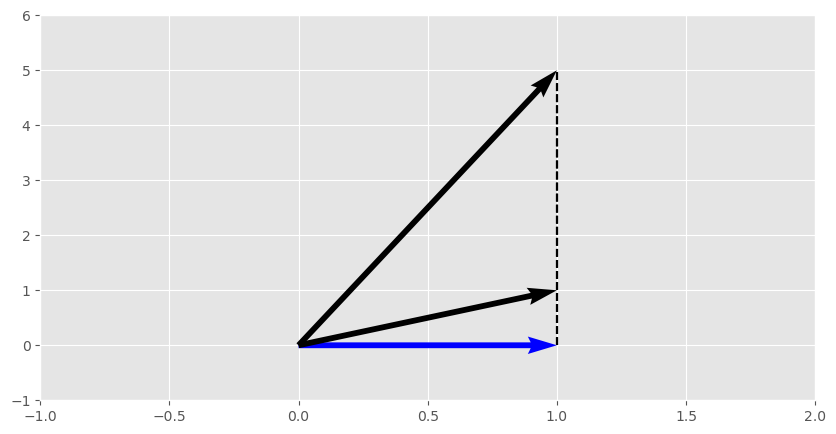
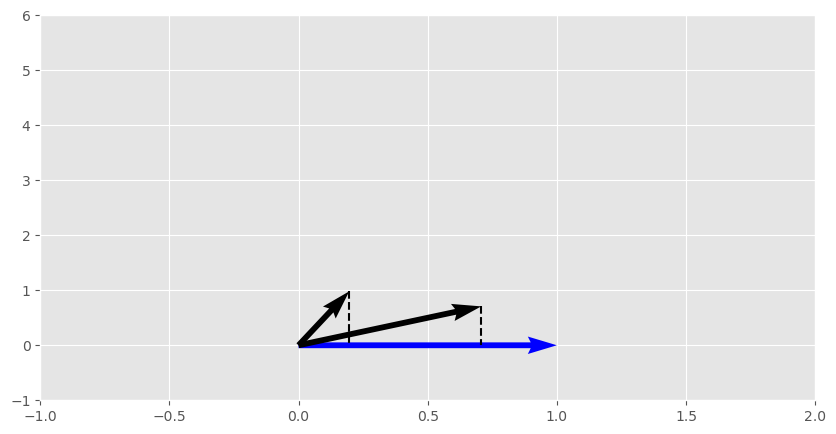
From this geometric standpoint, the multiplication occurs between the magnitude of one of the vectors and the projection of the other vector onto it. Looking at the above “geometric” formula, the vector that is being projected is the hypotenuse of a right triangle, while the projection is the adjacent side to the angle $\theta $, with $\cos (\theta) $ representing their proportion.
As this projection operation is symmetric between the two vectors, the dot product is commutative: $ x^Ty = y^Tx$
The angle between two vectors is useful in assessing their similarity, with similar vectors generally having smaller angles between them, i.e. pointing in a similar direction.
When assessing vector similarity, the dot product can be used as a shorthand for calculating the full angle. The dot product is equal to 0 if the two vectors are orthogonal. If the angle between the two vectors is acute, the dot product is positive, and negative if the the angle is obtuse.
The raw dot product is not a perfect proxy for the vector angle. For example, products $ \begin{bmatrix}1 \\ 1\end{bmatrix} \cdot \begin{bmatrix}1 \\ 0\end{bmatrix}$ and $ \begin{bmatrix}1 \\ 5\end{bmatrix} \cdot \begin{bmatrix}1 \\ 0\end{bmatrix}$ are both equal to 1 (and result in the same projection), yet the angles between these two vector pairs are wildly different (45° and ~79°).

This can be addressed by normalizing vectors by their magnitude prior to multiplication. This makes the dot product proportional to the angle between them. For the above example, the normalized dot product is 0.71 and 0.2, respectively.

The angle (in radians) between two vectors can be calculated by rearranging the geometric representation of the dot product: $$ \theta = \arccos(\frac{a \cdot b}{\Vert a \Vert \cdot \Vert b \Vert}) $$
In practice, calculating the actual angle is not necessary to assess vector similarity, as we can stop at just calculating the cosine of the angle (i.e., save ourselves the costly arccos operation). This is commonly referred to as the cosine similarity: $$ \cos (\theta) = \frac{a \cdot b}{\Vert a \Vert \cdot \Vert b \Vert} $$

The outer product

$$ x \otimes y = xy^T = \begin{bmatrix}x_1 \\ x_2 \end{bmatrix} \begin{bmatrix}y_1 & y_2 & y_3\end{bmatrix} = \begin{bmatrix} x_1y_1 & x_1y_2 & x_1y_3 \\ x_2y_1 & x_2y_2 & x_2y_3 \\ \end{bmatrix} $$

The outer product results in a matrix where each element of one vector gets multiplied by each element of the other. Due to this, it is also sometimes called the tensor product.
The utility of the outer product is a lot more niche than of the inner product, so I will omit the details in this review of the basics.

The cross product

Unlike the inner and outer products, the cross product is not just a special case of matrix multiplication. It is an operation that has a flavor of a vector product, but is more useful from the geometric standpoint.

$$ a \times b = \Vert a \Vert \Vert b \Vert \sin (\theta) n $$

where n is a unit vector perpendicular to the plane containing a and b.

Given that a and b are linearly independent, the cross product is a vector that is orthogonal to both input vectors.
The magnitude of the cross product is the area of the parallelogram where vectors a and b represent its sides.

Hadamard product

A quick mention on another “special” product, which is not just a special case of tensor multiplication. Hadamard product is the element-wise multiplication that is used less frequently in linear algebra. $$ (A \odot B)_{i,j} = (A)_{ij} (B)_{ij} $$

It takes two tensors of the same size and returns a tensor of the same size where each element is the product of corresponding elements from the original tensors.

Inverse of a matrix

An inverse of a square matrix “undoes” the transformation that it represents: $ A^{-1}A = I = AA^{-1}$
In the definition above, I represents the identity matrix, such that AI = A = IA. $$ I = \begin{cases} 1 & i=j \\ 0 & i \not = j \end{cases} $$
To make an analogy, an inverse of a matrix is like a reciprocal to a number.
Inverses are central to solving systems of linear equations. Recall that a such a system can be represented as $ A\vec{x} = \vec{b} $. This can be viewed as applying a transformation A to an unknown vector x such that it lands on a known vector b. Thus, to find x we just need to “undo” the transformation that is represented by matrix A and apply it to b: $$ \vec x = A^{-1} \vec b $$
There are various ways of finding an inverse of a matrix (e.g., Gaussian elimination), which are out of scope of this note.
Not all matrices have inverses:
- An invertible matrix must be square. This fact plays nicely with the condition that to solve a system of linear equations, you need at least as many equations as unknowns.
- The determinant of the matrix must be non-zero (more on that in the next section).

The Determinant

The determinant represents the “volume” of the n-dimensional parallelotope (parallelogram in 2D, parallelepiped in 3D) formed by the column vectors of the matrix.
There are various ways of calculating the determinant (e.g., Leibniz formula), depending on the dimensions of the matrix, but it generally boils down to calculating the “product of the diagonal elements minus the product of the off-diagonal elements”.
The determinant gives you an idea on what the transformation does to the vector space. If we consider a given matrix as the updated basis vectors of a space, then the determinant tells us how the volume defined by the basis vectors (where each dimension starts at 1) changes after the transformation.
- When the determinant is less than one, the space is generally squished, when it is more than 1, the space is generally expanded.
- If the determinant is 1, then the space does not change. This could represent the identity matrix (where nothing happens) or a transformation where the volume of the space is preserved, like rotation.
- When the determinant is zero, it signifies that one or more dimensions of the space collapse on themselves.
A zero determinant indicates that the columns (or rows) of the matrix are linearly dependent. In the context of solving a system of linear equations, this means that the system is either inconsistent (no solution) or has infinitely many solutions. You could imagine that inverting the collapse of a space creates situations where infinitely many points in the “new” dimension arise from a single point of an “old dimension”.
Thus, a matrix with a zero determinant is non-invertible (sometimes also called singular).

Eigenvectors and Eigenvalues

An eigenvector of a square matrix is a non-zero vector that, when multiplied by the matrix, results in a scaled version of itself without changing directions: $$ A \vec{v} = \lambda \vec{v} $$ where λ is the eigenvalue, or the scaling factor of the eigenvector.
When we view a matrix as a transformation, an eigenvector represents a direction towards which the space transforms as a whole. So in applications where a transformation is applied repeatedly, the largest eigenvalue defines the behavior of the system after multiple transformations, i.e. it’s steady state.
When dealing with rotation transformations, the eigenvectors can help identify the axes of these rotations.